Work with GeoJSON and Create the Map

Get the GeoJSON File

Next, we need a GeoJSON file with zip codes matching (or at least overlapping with) the ones in the CSV file. There’s one ready for you, which you can download here.

Reformat the GeoJSON

GeoJSON comes to us in the standard format:

{
    "type": "FeatureCollection",
    "features": [{
        "type": "Feature",
        "properties": {
            "kind": "ZIP Code Tabulation Area (2012)",
            "external_id": "90001",
            "name": "90001",
            "slug": "90001-zip-code-tabulation-area-2012",
            "set": "/1.0/boundary-set/zip-code-tabulation-areas-2012/",
            "metadata": {
                "AWATER10": 0,
                "CLASSFP10": "B5",
                "ALAND10": 9071359,
                "INTPTLAT10": "+33.9740268",
                "FUNCSTAT10": "S",
                "ZCTA5CE10": "90001",
                "MTFCC10": "G6350",
                "GEOID10": "90001",
                "INTPTLON10": "-118.2495088"
            },
            "resource_uri": "/1.0/boundary/90001-zip-code-tabulation-area-2012/"
        },
        "geometry": {
            "type": "MultiPolygon",
            "coordinates": [
                [
                    [
                        [-118.265151, 33.970249],
                        [-118.265166, 33.974735],
                        [-118.262969, 33.974746],
                        [-118.262981, 33.981836],
                        [-118.265174, 33.981828],
                        [-118.265185, 33.989227],
                        [-118.256436, 33.989317],
                        [-118.256436, 33.989498],
                        [-118.241159, 33.989422],
                        [-118.241126, 33.988174],
                        [-118.240505, 33.988158],
                        [-118.240502, 33.98867],
                        [-118.23899, 33.988664],
                        [-118.239021, 33.989403],
                        [-118.237918, 33.989393],
                        [-118.235685, 33.979486],
                        [-118.235352, 33.979534],
                        [-118.235105, 33.978705],
                        [-118.234324, 33.974732],
                        [-118.234685, 33.974731],
                        [-118.234432, 33.972967],
                        [-118.233915, 33.970674],
                        [-118.233561, 33.970731],
                        [-118.232835, 33.967469],
                        [-118.232995, 33.967467],
                        [-118.232405, 33.965314],
                        [-118.231371, 33.963268],
                        [-118.230013, 33.961768],
                        [-118.231885, 33.961565],
                        [-118.231599, 33.960146],
                        [-118.237366, 33.960152],
                        [-118.23737, 33.958521],
                        [-118.237943, 33.958518],
                        [-118.237949, 33.96015],
                        [-118.24499, 33.960148],
                        [-118.244994, 33.959648],
                        [-118.246648, 33.959637],
                        [-118.246653, 33.959177],
                        [-118.247237, 33.959175],
                        [-118.247225, 33.9597],
                        [-118.253962, 33.959701],
                        [-118.253959, 33.960162],
                        [-118.258573, 33.96016],
                        [-118.258575, 33.959577],
                        [-118.260754, 33.959772],
                        [-118.260753, 33.960149],
                        [-118.265118, 33.96013],
                        [-118.265139, 33.966482],
                        [-118.264629, 33.966483],
                        [-118.264607, 33.967438],
                        [-118.265142, 33.967395],
                        [-118.265151, 33.970249]
                    ]
                ]
            ]
        }
    }, ...]
}

Standard GeoJSON works well in most applications, but it’s problematic for custom maps in CRM Analytics. The problem isn’t in displaying the map; it occurs when you try to display data using the map chart. That’s because CRM Analytics looks for an ID at the same level as the "type": "Feature" node that matches an ID in the data. That’s how it knows to match a row from the CSV file to a particular zip-code area on the map. In fact, that ID property has to be named "id"!

In this example, the obvious ID to use is the zip code value itself. The fix is to move the key up one level, or just “flatten” the GeoJSON by moving everything under "properties" up one level. Let’s use our coding skills to see how we might accomplish this!

For the Los Angeles zip codes, create a script or use a fancy regular-expressions formula to move "external_id" up one level so it’s a child of "features".
Be sure to rename the new key-value node "id". The value of each "id" will be a zip code, to match the zip codes in your dataset's Zipcode column.
If your script outputs a file with a new name, note the name of the file and its location. You need them when you upload the GeoJSON to Analytics.

For example, here’s a quick-and-dirty Python script that creates the "id" node at the same level as "type".

                #!/usr/bin/python
                import json
                import os
                os.chdir(os.path.expanduser('~/Downloads'))
                # standard geojson file
                f = open('test_la_zip_code_areas_2012.geojson', 'r')
                json_contents = json.loads(f.read())
                features = json_contents["features"]
                for i in features:
                    i["id"] = i["properties"]["external_id"]
                json_contents["features"] = features
                # Normalized geojson for Tableau map
                out_file = open("out_la_zip_code_areas_2012.json", "w")
                out_file.write(json.dumps(json_contents))
                out_file.close()

The quick-and-dirty script shown above strips the wrapper around the feature objects, so if you use it, restore the following:

{    
                                                                                                      "type": "FeatureCollection",
                                                                                                      "features": {[
                                                                                                          "comment" : "stuff that was output by the script goes here"
                                                                                                      ]}
                                                                                                  }

Now the GeoJSON looks something like this:

{
    "type": "FeatureCollection",
    "features": [{
        "type": "Feature",
        "properties": {
            "kind": "ZIP Code Tabulation Area (2012)",
            "external_id": "90001",
            ...
            },
            "resource_uri": "/1.0/boundary/90001-zip-code-tabulation-area-2012/"
        },
        "id": "90001",
        "geometry": {
            "type": "MultiPolygon",
            "coordinates": [
                [
                        [-118.265151, 33.970249],
                        ...
                    ]
                ]
            ]
        }
    }, ...]
}

Every id has the value of the actual zip code in the feature object that it’s a part of. Don't try to use this GeoJSON snippet—it's just a small part of the output you'll get!

Display the Data in a Custom Map

When you created the Los Angeles zip code dataset, you set the Zipcode column’s data type to dimension. This action makes it possible to group by zip code when you explore the data. After you group the data by zip code, you’ll visualize it in a custom map that shows L.A. zip codes. You’ll have to create the custom map based on a geoJSON file.

Let’s explore the zip code data in a lens and view it on the custom map.

On the Analytics Studio home page, click Browse and type la_zip_codes in the Search bar.
Click the dataset from the search results to explore it in a lens.
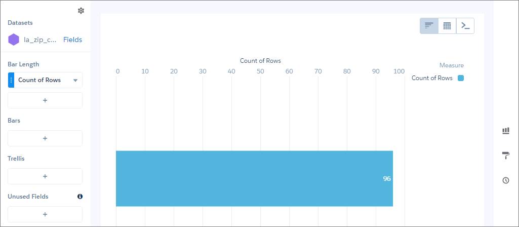
In the lens, click the Count of Rows measure, then Sum, then TotalWages to change the measure to Sum of TotalWages. Make sure to click the name of the measure you're changing, Count of Rows, in the Bar Length field.
Click the plus button in the Bars field, then select Zipcode to group by zip code.
To change the chart type to a map, click on the right and select the Map chart type (). The default map doesn’t show L.A. zip codes and therefore isn’t a good map for this data. Actually, none of the prebuilt map types can show data grouped by zip codes. Let’s create a custom map that can.
To create a custom map type, click , expand the Map section, and then next to the Map Type property.
In case you didn’t reformat your own GeoJSON file, we’ve reformatted one for you. Right-click this link and save the reformatted GeoJSON file to your local machine.
In the left pane of the New Map page, click Upload GeoJSON and upload the GeoJSON definition (custom_map_project_geojson.json) that you downloaded.

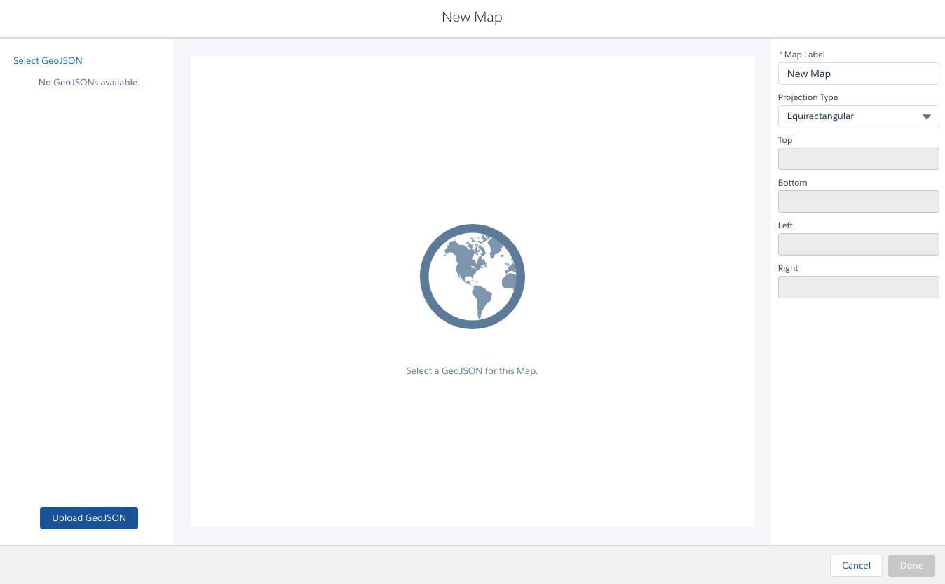
If there’s something wrong with the GeoJSON file that you uploaded, an error message appears (something like “Invalid GeoJSON”). Usually that means something went wrong with the reformatting.
In the Map Label field, enter L.A. Zipcodes.
In the Projection Type field, select Equirectangular as the default projection type for this map. You can override this setting in the widget properties for each chart widget that uses this custom map. Equirectangular is appropriate for simple geometric shapes such as floor plans, city blocks, or zip-code areas. Mercator is most suitable for traditional geographical maps. Use AlbersUSA for a map of the United States of America that includes Hawaii and Alaska near the rest of the United States. In the center pane, you could drag the handles of the map to change the boundaries, and zoom in on a particular region. The boundaries would show in the right pane. However, we won’t change the boundaries yet. We’ll look at them in more detail in a bit.
Click Done. Congratulations! You’ve created your first custom map. And isn’t it a beauty! You can now use this custom map type in other charts, including map, geo map, and bubble map charts.
To clip this lens to a dashboard in designer, click .
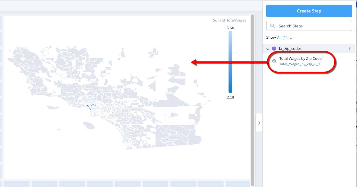
In the query naming dialog, enter Total Wages by Zip Code in the Display Label field, and click Clip to Designer.
In the dashboard designer, drag the new query onto the canvas. Adjust the size of the widget as necessary to be able to view the bar chart that appears. An unimpressive map appears with several colored zip-code areas where Los Angeles is found (those flyspecks approximately in the central part of the visible coast).
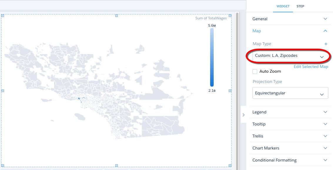
Select the map to display the widget properties.
In the widget properties, expand the Map section and notice that the new L. A. Zipcodes custom map is selected in the Map Type menu.
Save the dashboard, naming it Los Angeles Tax Data by Zip Code.

The problem with this map is that it includes zip code areas for all of Southern California, which means the Los Angeles area is much too small to be useful. We can fix that by creating a bounding box. We do that next.